HTB CTF Writeup: Bending the Output to Your Will

Challenge: Neural Net Power Distribution (AI/ML) Flag: HTB{b3nd1ng_*****_w1LL} Difficulty: Medium Category: AI / Machine Learning

The Scenario

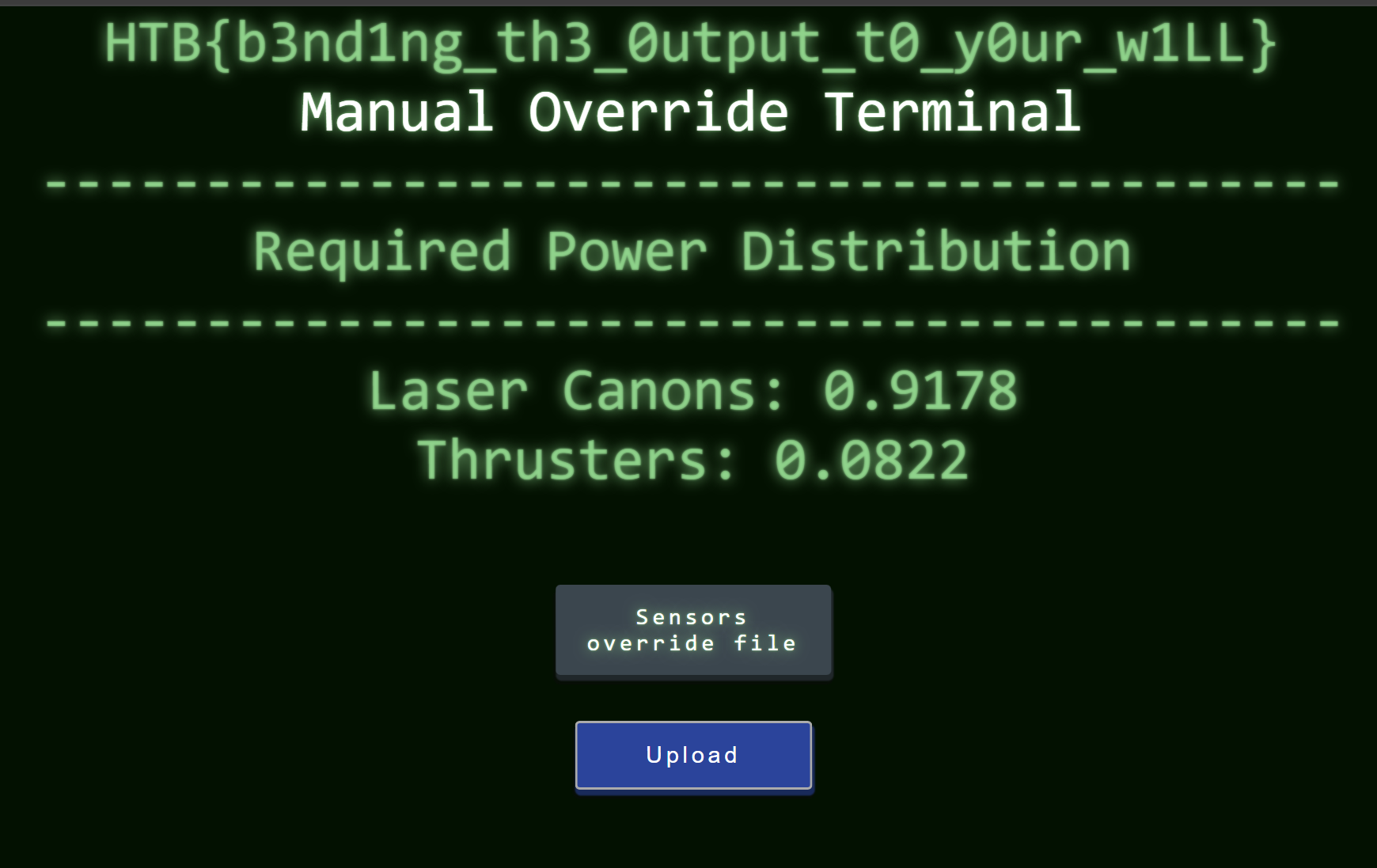
A spaceship’s autopilot has been destroyed by an electromagnetic cannon. To survive a meteor shower ahead, the pilot Ramona needs to manually balance power between the laser cannons (for destroying meteors) and the thrusters (for maneuvering). The onboard neural network verifies any new configuration, and it demands a very specific power split:

Laser Canons: 0.9178
Thrusters:    0.0822

Our job: craft a .npy file of “sensor values” that, when fed through the neural network, produces exactly that output — to within 99.99% accuracy.

What We’re Given

Two files:

• net.py — the neural network architecture
• model.pth — the trained model weights

The network is a small CNN (convolutional neural network) that takes a single-channel grayscale image and outputs two probabilities via softmax:

python

class net(nn.Module):
    def __init__(self):
        super(net, self).__init__()
        self.layer1 = nn.Sequential(
            nn.Conv2d(1, 16, kernel_size=3, padding=0, stride=2),
            nn.ReLU(),
            nn.MaxPool2d(2)
        )
        self.layer2 = nn.Sequential(
            nn.Conv2d(16, 32, kernel_size=3, padding=0, stride=2),
            nn.ReLU(),
            nn.MaxPool2d(2)
        )
        self.fc1 = nn.Linear(5408, 10)
        self.fc2 = nn.Linear(10, 2)
        self.relu = nn.ReLU()

    def forward(self, x):
        out = self.layer1(x)
        out = self.layer2(out)
        out = out.view(out.size(0), -1)
        out = self.relu(self.fc1(out))
        out = self.fc2(out)
        out = torch.softmax(out, dim=1)
        return out

Step 1: Understanding the Architecture

Before we can craft an input, we need to know what shape it expects. The fully-connected layer fc1 takes 5,408 inputs, which equals 32 channels × 13 × 13 spatial dimensions — that’s the output of the second conv block. Working backwards through the convolutions and pooling layers, a 224×224 input produces exactly that shape:

Input:  (1, 1, 224, 224)     ← 1 grayscale 224×224 image
  ↓ Conv2d(1→16, k=3, s=2) + ReLU + MaxPool(2)
        (1, 16, 55, 55)
  ↓ Conv2d(16→32, k=3, s=2) + ReLU + MaxPool(2)
        (1, 32, 13, 13)
  ↓ Flatten
        (1, 5408)
  ↓ Linear(5408→10) + ReLU
        (1, 10)
  ↓ Linear(10→2) + Softmax
        (1, 2)               ← [P(lasers), P(thrusters)]

A quick sanity check with random noise confirms the model runs cleanly on 224×224 input:

python

model = torch.load('model.pth', map_location='cpu', weights_only=False)
model.eval()

x = torch.randn(1, 1, 224, 224)
print(model(x))
# tensor([[4.3702e-05, 9.9996e-01]])  ← random noise → nearly all power to thrusters

Random inputs push the output heavily toward class 1 (thrusters). We need to sculpt the input so the output lands on [0.9178, 0.0822] instead.

Step 2: The Key Insight — Reverse Optimization

Normally when training a neural network, you freeze the input data and optimize the weights using gradient descent. Here we do the exact opposite: the weights are frozen (loaded from model.pth), and we optimize the input pixels instead.

This is the same technique used in adversarial examples and neural style transfer. PyTorch makes it straightforward because requires_grad=True can be set on any tensor, not just model parameters.

Step 3: The Attack

The approach is elegant in its simplicity:

python

# Define what we want the output to be
target = torch.tensor([[0.9178, 0.0822]])

# Start with random noise — this is what we'll optimize
input_tensor = torch.randn(1, 1, 224, 224, requires_grad=True)

# Use Adam optimizer, but on the INPUT, not the model weights
optimizer = torch.optim.Adam([input_tensor], lr=0.01)

for i in range(2000):
    optimizer.zero_grad()
    output = model(input_tensor)

    # Loss = how far is the output from our target?
    loss = ((output - target) ** 2).sum()

    # Backpropagate gradients all the way to the input pixels
    loss.backward()

    # Nudge each pixel to reduce the loss
    optimizer.step()

Each iteration, PyTorch computes the gradient of the loss with respect to every single input pixel: “if I increase this pixel by a tiny amount, does the output move closer to or further from [0.9178, 0.0822]?” Then Adam adjusts all 50,176 pixels simultaneously.

The optimization converges remarkably fast — within about 300 steps the output hits the target with error less than 0.0001:

Step   0: output=[0.00005, 0.99995]  error=0.91775   ← random noise, way off
Step 100: output=[0.89412, 0.10588]  error=0.02368   ← getting close
Step 200: output=[0.91693, 0.08307]  error=0.00087   ← almost there
Step 299: output=[0.91777, 0.08223]  error=0.00003   ← within tolerance ✓

Step 4: Saving and Uploading

A critical detail: the server expected a .npy file with shape (224, 224) — a bare 2D array, not wrapped in batch or channel dimensions. This makes sense thematically: you’re uploading a flat grid of sensor readings, and the server handles the reshaping internally.

python

import numpy as np
arr = input_tensor.detach().squeeze().numpy()  # (224, 224)
np.save('config.npy', arr.astype(np.float32))

Upload config.npy → the neural network verifies the power distribution matches → flag appears.

The Flag

HTB{b3nd1ng_th3_0utput_t0_y0ur_w1LL}

Takeaways

This challenge demonstrates a fundamental property of differentiable systems: if you can compute gradients through a model, you can optimize anything that feeds into it. The same principle underlies adversarial attacks on image classifiers, prompt injection on language models, and neural style transfer in art. The model’s weights are just fixed constraints — the input space is yours to explore.